Tangent skim modes

When tangent skimming is enabled, the following models are available to calculate suitable peak areas:

Exponential
New exponential
Standard (automatically chooses exponential or straight line calculations for the best fit)
Straight
Gaussian

If you need to quantitate signals that include skimmed peaks or shoulder peaks, consider evaluating peak height instead of peak area.

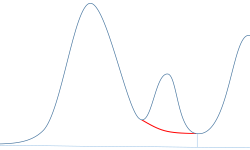
Exponential Skim

This skim model draws a curve using an exponential equation through the start and end of the child peak. The curve passes individually under each child peak that follows the parent peak.

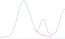
New Exponential Skim

This skim model draws a curve using an exponential equation. It approximates the leading or trailing edge on the parent peak signal. The curve passes under one or more child peaks. More than one child peak can be skimmed using the same exponential model; all peaks after the first child peak are separated by drop lines, beginning at the end of the first child peak, and are dropped only to the skim curve.

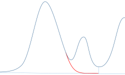
Gaussian Skim

This skim model uses the same equation as the New Exponential Skim; however, it searches higher up on the parent peak to find the best fit, and it approximates the leading or trailing edge on the parent peak baseline. Therefore, Gaussian skim usually calculates a larger area than the New Exponential skim.

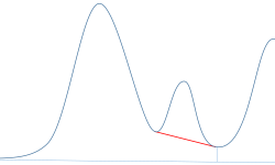
Straight Line Skim

This skim model draws a straight line through the start and end of a child peak. The height of the start of a tail rider peak (or end of a front rider peak, respectively) might be corrected for the parent peak slope.

Standard Skims

This default method is a combination of exponential and straight line calculations for the best fit.

The switch from an exponential to a linear calculation is performed in a way that eliminates abrupt discontinuities of heights or areas.

When the signal is well above the baseline, the tail-fitting calculation is exponential.
When the signal is within the baseline envelope, the tail fitting calculation is a straight line.

The combination calculations are reported as exponential or straight tangent skim.